Robustness

---

1 Custom functions

rm(list = ls())

fpackage.check <- function(packages) {
    lapply(packages, FUN = function(x) {
        if (!require(x, character.only = TRUE)) {
            install.packages(x, dependencies = TRUE)
            library(x, character.only = TRUE)
        }
    })
}

fsave <- function(x, file = NULL, location = "./data/processed/") {
    ifelse(!dir.exists("data"), dir.create("data"), FALSE)
    ifelse(!dir.exists("data/processed"), dir.create("data/processed"), FALSE)
    if (is.null(file))
        file = deparse(substitute(x))
    datename <- substr(gsub("[:-]", "", Sys.time()), 1, 8)
    totalname <- paste(location, file, "_", datename,  ".rda", sep = "")
    save(x, file = totalname)  #need to fix if file is reloaded as input name, not as x. 
}

fload <- function(filename) {
    load(filename)
    get(ls()[ls() != "filename"])
}

fshowdf <- function(x, ...) {
    knitr::kable(x, digits = 3, "html", ...) %>%
        kableExtra::kable_styling(bootstrap_options = c("striped", "hover")) %>%
        kableExtra::scroll_box(width = "100%", height = "300px")
}

colorize <- function(x, color) {sprintf("<span style='color: %s;'>%s</span>", color, x) }

---

2 Packages

packages = c("ggplot2", "ggpubr", "tidyverse", "RColorBrewer", "stringdist", "stringi", "future.apply",
    "gamlss", "gamlss.dist", "gamlss.tr", "splines", "splines2", "psych", "MASS", "dplyr", "flextable",
    "fastDummies", "fixest", "ggtext")

# load dplyr last otherwise conflict with select from MASS
fpackage.check(packages)

---

3 Input

We use three processed datasets.

• 20240717df_ppf.rda: person period file for main analysis
  
• 20240717df_pubs.rda: publications for descriptives
  
• 20240711linked_pubs_oa_fields.rda: publications linked to fields

df_ppf <- fload(file = "./data/processed/20240717df_ppf.rda")

df_pubs <- fload(file = "./data/processed/20240717df_pubs.rda")

df_fields <- fload(file = "./data/processed/20240711linked_pubs_oa_fields.rda")

---

4 Data wrangling

4.1 Domain

I will use all publications. Also the publications of 2020 and later, as I think this indicates the field/domain the author was working in during Covid.

I don’t pick the top domain, but calculate a percentage within domain. This does imho more justice to multidisciplinary and also takes into account possible arbitrariness in the black box of openalex domain identifier.

domain <- df_fields %>% dplyr::select("domain", "id") %>% #select conflicts with MASS
                filter(!is.na(domain)) %>%
                mutate(domain2 = as.numeric(as.factor(domain))) %>% #make numeric of domain variable
                group_by(id)  %>%
                mutate(npubs_domain = n(), #number of publications domain is based
                       health_domain = sum(domain2 == 1) / npubs_domain, #domain as proportions
                       life_domain = sum(domain2 == 2) / npubs_domain,
                       physical_domain = sum(domain2 == 3) / npubs_domain,
                       social_domain = sum(domain2 == 4) / npubs_domain) %>%
                ungroup() %>% #only keep one record per id
                mutate(id.dup =ifelse(duplicated(id), 1,0)) %>% 
                filter(id.dup == 0) %>%
                dplyr::select("id", "npubs_domain", "health_domain", "life_domain", "physical_domain", "social_domain")

#describe(domain)

add to our df_ppf

df_ppf <- df_ppf %>%
    left_join(domain)

4.2 Gender

df_gender <- df_pubs %>%
    ungroup() %>%
    mutate(id.dup = ifelse(duplicated(id), 1, 0)) %>%
    filter(id.dup == 0) %>%
    dplyr::select("id", "gender_2", "firstname", "lastname") %>%
    mutate(gender2 = ifelse(is.na(firstname) & is.na(gender_2), 3, gender_2))

df_gender$gender2[is.na(df_gender$gender2)] <- 4
df_gender$gender2 <- as.factor(df_gender$gender2)
levels(df_gender$gender2) <- c("men", "women", "no first name", "missing")

df_ppf <- df_ppf %>%
    left_join(df_gender)

4.3 Time (career age)

df_ppf$time <- df_ppf$pub_year - df_ppf$phd_year

df_ppf$covid <- as.numeric(df_ppf$pub_year == 2020 | df_ppf$pub_year == 2021)
df_ppf$covid2020 <- as.numeric(df_ppf$pub_year == 2020)
df_ppf$covid2021 <- as.numeric(df_ppf$pub_year == 2021)

df_ppf$age25 <- as.numeric(df_ppf$phd_year > 2010)
df_ppf$age25_2 <- as.numeric(df_ppf$phd_year > 2015)

df_ppf$phd_year0 <- df_ppf$phd_year - 1990

df_ppf$stem <- ifelse((df_ppf$field == "Biological and Health Sciences" | df_ppf$field == "Physical and Mathematical Sciences" |
    df_ppf$field == "Engineering" | df_ppf$field == "Agricultural Sciences"), "STEM-M", ifelse(df_ppf$field ==
    "missing", "missing", "NON-STEM-M"))

df_ppf$ethnicity <- as.factor(df_ppf$ethnicity)
df_ppf$ethnicity <- relevel(df_ppf$ethnicity, 2)
# levels(df_ppf$ethnicity)

df_ppf$multidisc <- 1 - (df_ppf$health_domain^2 + df_ppf$life_domain^2 + df_ppf$physical_domain^2 + df_ppf$social_domain^2)

---

5 Robustness checks

5.1 Model 2 separate per domain

5.1.1 Strict selection

I am currently making strict selections on domain. Namely, authors who only publish in a specific domain. A different strategy would be to use >.5 as criteria or classifying scholars based on highest score across the domains.

df3 <- df_ppf[, c("npubs", "npubs_a", "npubs_first_a", "npubs_last_a", "time", "id", "covid", "covid2020",
    "covid2021", "gender2", "phd_year0", "ethnicity", "uni", "health_domain", "life_domain", "physical_domain",
    "social_domain")]
df3 <- na.omit(df3)

knots5 <- quantile(df3$time, probs = seq(0, 1, 0.25))[2:4]
con <- gamlss.control(n.cyc = 150)


df3_d1 <- df3[df3$health_domain == 1, ]
df3_d2 <- df3[df3$life_domain == 1, ]
df3_d3 <- df3[df3$physical_domain == 1, ]
df3_d4 <- df3[df3$social_domain == 1, ]

m2_d1 <- gamlss(npubs ~ bSpline(time, knots = knots5, df = 3) + phd_year0 + covid + gender2 + ethnicity +
    uni + covid * gender2, data = df3_d1, family = BNB, control = con)
fsave(m2_d1, "m2_d1")
sm2_d1 <- summary(m2_d1)
fsave(sm2_d1, "sm2_d1")

m2_d2 <- gamlss(npubs ~ bSpline(time, knots = knots5, df = 3) + phd_year0 + covid + gender2 + ethnicity +
    uni + covid * gender2, data = df3_d2, family = BNB, control = con)
fsave(m2_d2, "m2_d2")
sm2_d2 <- summary(m2_d2)
fsave(sm2_d2, "sm2_d2")

m2_d3 <- gamlss(npubs ~ bSpline(time, knots = knots5, df = 3) + phd_year0 + covid + gender2 + ethnicity +
    uni + covid * gender2, data = df3_d3, family = BNB, control = con)
fsave(m2_d3, "m2_d3")
sm2_d3 <- summary(m2_d3)
fsave(sm2_d3, "sm2_d3")

m2_d4 <- gamlss(npubs ~ bSpline(time, knots = knots5, df = 3) + phd_year0 + covid + gender2 + ethnicity +
    uni + covid * gender2, data = df3_d4, family = BNB, control = con)
fsave(m2_d4, "m2_d4")
sm2_d4 <- summary(m2_d4)
fsave(sm2_d4, "sm2_d4")

names <- c("Intercept: mu", "bSpline(time, knots = knots5, df = 3)1", "bSpline(time, knots = knots5, df = 3)2",
    "bSpline(time, knots = knots5, df = 3)3", "bSpline(time, knots = knots5, df = 3)4", "bSpline(time, knots = knots5, df = 3)5",
    "bSpline(time, knots = knots5, df = 3)6", "PhD-cohort", "COVID-19 years", "gender: women", "gender: no first name",
    "gender: missing", "ethnicity: minority I", "ethnicity: minority II", "ethnicity: missing", "university: LU",
    "university: RU", "university: RUG", "university: TUE", "university: TI", "university: UM", "university: UT",
    "university: UU", "university: UvA", "university: VU", "university: WUR", "COVID*women", "COVID*no first name",
    "COVID*missing", "Intercept: sigma", "Intercept: nu")
rownames(sm2_d1) <- names

names <- c("Intercept: mu", "bSpline(time, knots = knots5, df = 3)1", "bSpline(time, knots = knots5, df = 3)2",
    "bSpline(time, knots = knots5, df = 3)3", "bSpline(time, knots = knots5, df = 3)4", "bSpline(time, knots = knots5, df = 3)5",
    "bSpline(time, knots = knots5, df = 3)6", "PhD-cohort", "COVID-19 years", "gender: women", "gender: no first name",
    "gender: missing", "ethnicity: minority I", "ethnicity: minority II", "ethnicity: missing", "university: LU",
    "university: RU", "university: RUG", "university: UM", "university: UT", "university: UU", "university: UvA",
    "university: VU", "university: WUR", "COVID*women", "COVID*no first name", "COVID*missing", "Intercept: sigma",
    "Intercept: nu")
rownames(sm2_d2) <- names

names <- c("Intercept: mu", "bSpline(time, knots = knots5, df = 3)1", "bSpline(time, knots = knots5, df = 3)2",
    "bSpline(time, knots = knots5, df = 3)3", "bSpline(time, knots = knots5, df = 3)4", "bSpline(time, knots = knots5, df = 3)5",
    "bSpline(time, knots = knots5, df = 3)6", "PhD-cohort", "COVID-19 years", "gender: women", "gender: no first name",
    "gender: missing", "ethnicity: minority I", "ethnicity: minority II", "ethnicity: missing", "university: LU",
    "university: RU", "university: RUG", "university: TUD", "university: TUE", "university: UM", "university: UT",
    "university: UU", "university: UvA", "university: VU", "university: WUR", "COVID*women", "COVID*no first name",
    "COVID*missing", "Intercept: sigma", "Intercept: nu")
rownames(sm2_d3) <- names

names <- c("Intercept: mu", "bSpline(time, knots = knots5, df = 3)1", "bSpline(time, knots = knots5, df = 3)2",
    "bSpline(time, knots = knots5, df = 3)3", "bSpline(time, knots = knots5, df = 3)4", "bSpline(time, knots = knots5, df = 3)5",
    "bSpline(time, knots = knots5, df = 3)6", "PhD-cohort", "COVID-19 years", "gender: women", "gender: no first name",
    "gender: missing", "ethnicity: minority I", "ethnicity: minority II", "ethnicity: missing", "university: LU",
    "university: RU", "university: RUG", "university: TUD", "university: TUE", "university: TI", "university: UM",
    "university: UT", "university: UU", "university: UvA", "university: VU", "university: WUR", "COVID*women",
    "COVID*no first name", "COVID*missing", "Intercept: sigma", "Intercept: nu")
rownames(sm2_d4) <- names


fshowdf(sm2_d1)
fshowdf(sm2_d2)
fshowdf(sm2_d3)
fshowdf(sm2_d4)

	Estimate	Std. Error	t value	Pr(>|t|)
Intercept: mu	1.550	0.081	19.219	0.000
bSpline(time, knots = knots5, df = 3)1	-0.733	0.110	-6.681	0.000
bSpline(time, knots = knots5, df = 3)2	-0.894	0.093	-9.604	0.000
bSpline(time, knots = knots5, df = 3)3	-1.150	0.096	-12.033	0.000
bSpline(time, knots = knots5, df = 3)4	-1.094	0.172	-6.372	0.000
bSpline(time, knots = knots5, df = 3)5	-1.004	0.284	-3.539	0.000
bSpline(time, knots = knots5, df = 3)6	-2.475	0.385	-6.427	0.000
PhD-cohort	-0.033	0.003	-10.614	0.000
COVID-19 years	-0.485	0.080	-6.089	0.000
gender: women	-0.240	0.036	-6.722	0.000
gender: no first name	0.835	0.174	4.812	0.000
gender: missing	0.411	0.405	1.016	0.310
ethnicity: minority I	0.094	0.159	0.589	0.556
ethnicity: minority II	0.016	0.068	0.241	0.810
ethnicity: missing	-0.242	0.066	-3.660	0.000
university: LU	-0.146	0.354	-0.412	0.680
university: RU	0.278	0.045	6.205	0.000
university: RUG	0.382	0.152	2.519	0.012
university: TUE	-1.607	0.461	-3.482	0.000
university: TI	0.629	0.174	3.619	0.000
university: UM	0.309	0.056	5.519	0.000
university: UT	-0.299	0.103	-2.897	0.004
university: UU	0.273	0.062	4.427	0.000
university: UvA	0.296	0.079	3.733	0.000
university: VU	0.391	0.095	4.130	0.000
university: WUR	0.666	0.089	7.506	0.000
COVID*women	-0.125	0.109	-1.142	0.254
COVID*no first name	0.531	0.569	0.934	0.350
COVID*missing	0.026	0.809	0.032	0.974
Intercept: sigma	-1.642	0.093	-17.620	0.000
Intercept: nu	-1.426	0.175	-8.161	0.000

	Estimate	Std. Error	t value	Pr(>|t|)
Intercept: mu	1.711	0.145	11.783	0.000
bSpline(time, knots = knots5, df = 3)1	-0.782	0.171	-4.568	0.000
bSpline(time, knots = knots5, df = 3)2	-0.879	0.127	-6.896	0.000
bSpline(time, knots = knots5, df = 3)3	-1.184	0.138	-8.580	0.000
bSpline(time, knots = knots5, df = 3)4	-0.757	0.199	-3.801	0.000
bSpline(time, knots = knots5, df = 3)5	-1.305	0.258	-5.051	0.000
bSpline(time, knots = knots5, df = 3)6	-1.509	0.260	-5.796	0.000
PhD-cohort	-0.058	0.004	-14.754	0.000
COVID-19 years	-0.571	0.083	-6.863	0.000
gender: women	-0.096	0.049	-1.972	0.049
gender: no first name	-0.649	0.337	-1.927	0.054
gender: missing	-0.608	1.061	-0.573	0.567
ethnicity: minority I	-0.412	0.237	-1.738	0.082
ethnicity: minority II	-0.260	0.079	-3.299	0.001
ethnicity: missing	-0.271	0.059	-4.564	0.000
university: LU	0.031	0.256	0.121	0.904
university: RU	0.129	0.103	1.246	0.213
university: RUG	1.013	0.172	5.892	0.000
university: UM	0.018	0.129	0.140	0.889
university: UT	-0.471	0.351	-1.342	0.180
university: UU	-0.029	0.128	-0.226	0.821
university: UvA	0.313	0.106	2.956	0.003
university: VU	0.391	0.125	3.115	0.002
university: WUR	0.588	0.093	6.355	0.000
COVID*women	0.200	0.120	1.662	0.097
COVID*no first name	-0.359	0.851	-0.422	0.673
COVID*missing	-34.642	70710.678	0.000	1.000
Intercept: sigma	-2.510	0.127	-19.708	0.000
Intercept: nu	-0.958	0.147	-6.511	0.000

	Estimate	Std. Error	t value	Pr(>|t|)
Intercept: mu	2.118	0.310	6.842	0.000
bSpline(time, knots = knots5, df = 3)1	-0.702	0.102	-6.848	0.000
bSpline(time, knots = knots5, df = 3)2	-0.740	0.087	-8.547	0.000
bSpline(time, knots = knots5, df = 3)3	-0.971	0.087	-11.184	0.000
bSpline(time, knots = knots5, df = 3)4	-0.262	0.147	-1.783	0.075
bSpline(time, knots = knots5, df = 3)5	-1.068	0.216	-4.934	0.000
bSpline(time, knots = knots5, df = 3)6	-1.225	0.237	-5.164	0.000
PhD-cohort	-0.035	0.003	-11.758	0.000
COVID-19 years	-0.570	0.058	-9.880	0.000
gender: women	0.039	0.041	0.957	0.339
gender: no first name	-0.287	0.155	-1.849	0.064
gender: missing	0.600	0.153	3.910	0.000
ethnicity: minority I	-0.232	0.118	-1.962	0.050
ethnicity: minority II	-0.214	0.052	-4.108	0.000
ethnicity: missing	-0.026	0.039	-0.674	0.500
university: LU	0.096	0.318	0.301	0.763
university: RU	0.188	0.304	0.619	0.536
university: RUG	0.685	0.331	2.066	0.039
university: TUD	0.594	0.317	1.878	0.060
university: TUE	0.459	0.303	1.518	0.129
university: UM	-1.017	0.434	-2.347	0.019
university: UT	-0.236	0.302	-0.781	0.435
university: UU	0.154	0.302	0.510	0.610
university: UvA	0.380	0.302	1.259	0.208
university: VU	-0.012	0.305	-0.040	0.968
university: WUR	0.014	0.303	0.047	0.963
COVID*women	0.135	0.109	1.245	0.213
COVID*no first name	-0.355	0.738	-0.481	0.630
COVID*missing	-0.412	0.749	-0.549	0.583
Intercept: sigma	-0.376	0.049	-7.695	0.000
Intercept: nu	-0.788	0.133	-5.926	0.000

	Estimate	Std. Error	t value	Pr(>|t|)
Intercept: mu	1.232	0.105	11.711	0.000
bSpline(time, knots = knots5, df = 3)1	-0.438	0.079	-5.560	0.000
bSpline(time, knots = knots5, df = 3)2	-0.478	0.063	-7.597	0.000
bSpline(time, knots = knots5, df = 3)3	-0.670	0.063	-10.644	0.000
bSpline(time, knots = knots5, df = 3)4	-1.006	0.108	-9.331	0.000
bSpline(time, knots = knots5, df = 3)5	-1.125	0.180	-6.256	0.000
bSpline(time, knots = knots5, df = 3)6	-2.696	0.255	-10.580	0.000
PhD-cohort	-0.044	0.002	-20.955	0.000
COVID-19 years	-0.571	0.056	-10.196	0.000
gender: women	-0.088	0.023	-3.814	0.000
gender: no first name	-0.327	0.107	-3.050	0.002
gender: missing	-0.146	0.295	-0.494	0.621
ethnicity: minority I	-0.103	0.104	-0.991	0.322
ethnicity: minority II	-0.184	0.046	-3.982	0.000
ethnicity: missing	-0.031	0.032	-0.949	0.343
university: LU	0.592	0.115	5.162	0.000
university: RU	0.570	0.097	5.887	0.000
university: RUG	0.855	0.099	8.620	0.000
university: TUD	0.235	0.539	0.435	0.663
university: TUE	0.178	0.167	1.065	0.287
university: TI	0.695	0.117	5.930	0.000
university: UM	0.661	0.099	6.698	0.000
university: UT	0.554	0.105	5.270	0.000
university: UU	0.469	0.103	4.540	0.000
university: UvA	0.677	0.096	7.029	0.000
university: VU	0.632	0.098	6.426	0.000
university: WUR	0.467	0.145	3.225	0.001
COVID*women	0.060	0.078	0.762	0.446
COVID*no first name	-0.190	0.401	-0.473	0.636
COVID*missing	1.200	0.615	1.950	0.051
Intercept: sigma	-1.887	0.080	-23.494	0.000
Intercept: nu	-1.643	0.185	-8.871	0.000

5.2 Fixed effects career age and person id

df3 <- df_ppf[, c("npubs", "npubs_a", "npubs_first_a", "npubs_last_a", "time", "pub_year", "id", "covid",
    "covid2020", "covid2021", "gender2", "phd_year0", "phd_year", "ethnicity", "uni", "life_domain",
    "physical_domain", "social_domain")]
df3 <- na.omit(df3)

df3$log_npubs <- log(df3$npubs + 1)
m_fe <- feols(log_npubs ~ 1 + covid + i(gender2, covid, ref = c("men")) | id + time, data = df3)
fshowdf(summary(m_fe)$coeftable)

	Estimate	Std. Error	t value	Pr(>|t|)
covid	-0.284	0.009	-33.260	0.000
gender2::women:covid	0.039	0.013	3.041	0.002
gender2::no first name:covid	-0.097	0.059	-1.643	0.100
gender2::missing:covid	0.026	0.103	0.249	0.804

Based on this modelling strategy we would conclude that women were significantly less negatively impacted by COVID-19 with respect to their absolute number of yearly articles.

5.3 Table 4

Staying close to modelling strategy of Madsen et al. (2022).

We do not use year of first pub to define career age but phd_year

df3 <- df_ppf[, c("npubs", "npubs_a", "npubs_first_a", "npubs_last_a", "time", "pub_year", "id", "covid",
    "covid2020", "covid2021", "gender2", "phd_year", "phd_year0", "ethnicity", "uni", "life_domain",
    "physical_domain", "social_domain")]

df3$log_npubs_a <- log(df3$npubs_a + 1)

df3_mid <- df3[df3$phd_year == 2008 | df3$phd_year == 2009 | df3$phd_year == 2010, ]
df3_early <- df3[df3$phd_year == 2014 | df3$phd_year == 2015 | df3$phd_year == 2016, ]

# remove missings on gender
df3_early <- df3_early[df3_early$gender2 == "men" | df3_early$gender2 == "women", ]
df3_mid <- df3_mid[df3_mid$gender2 == "men" | df3_mid$gender2 == "women", ]

df3_early$women <- ifelse(df3_early$gender2 == "women", 1, 0)
df3_mid$women <- ifelse(df3_mid$gender2 == "women", 1, 0)

5.3.1 observations

print("N_persons (early career)")
length(unique(df3_early$id))
print("N_observations (early career)")
nrow(df3_early)

print("N_persons (mid career)")
length(unique(df3_mid$id))
print("N_observations (mid career)")
nrow(df3_mid)

#> [1] "N_persons (early career)"
#> [1] 1310
#> [1] "N_observations (early career)"
#> [1] 8888
#> [1] "N_persons (mid career)"
#> [1] 1242
#> [1] "N_observations (mid career)"
#> [1] 14959

m_fe_e <- feols(log_npubs_a ~ 1 + i(pub_year, women, ref = "2019") | id + pub_year, data = df3_early)
m_fe_m <- feols(log_npubs_a ~ 1 + i(pub_year, women, ref = "2019") | id + pub_year, data = df3_mid)

5.3.2 fit measures

r2 <- c(fixest::r2(m_fe_e, "r2"), fixest::r2(m_fe_m, "r2"))  #overal r2
wr2 <- c(fixest::r2(m_fe_e, "wr2"), fixest::r2(m_fe_m, "wr2"))  #within r2

df_fitst4 <- data.frame(r2 = r2, wr2 = wr2)
# fsave(df_fitst4, 'df_fitst4')

smfee <- as.data.frame(coeftable(m_fe_e))
smfee$names <- rownames(smfee)
smfem <- as.data.frame(coeftable(m_fe_m))
smfem$names <- rownames(smfem)
res <- right_join(smfee, smfem, by = "names")
res <- res[order(res$names), ]

res <- res[, -c(3, 8)]
res <- res[, c(4, 1:3, 5:7)]
res$names <- c("year2009*women", "year2010*women", "year2011*women", "year2012*women", "year2013*women",
    "year2014*women", "year2015*women", "year2016*women", "year2017*women", "year2018*women", "year2020*women",
    "year2021*women", "year2022*women")

colnames(res) <- as.character(1:7)

# fsave(res, 'Table4_raw')
Table4_raw <- res

table4ft <- flextable(Table4_raw)  %>% add_header_row(values=c(" ", rep(c("B", "S.E.", "P"), 2)), top=FALSE) %>% delete_rows(i=1,part="header") %>% 
  #set_caption( "Fixed-Effects model for yearly article output (logtransformed; Gaussian)") %>% 
  add_footer_lines(value = c("Notes: \nFor reasons of parsimony, the estimates of the fixed effects are not shown: scholars; year. Scholars with missing values on gender were removed from the analysis.\nEarly career: N_observations 8,888; N_persons 1,310 \n Mid career: N_obervations 14,959; N_persons: 1,242")) %>%
   add_header_row(values = c(" ", "early career PhDs", "mid-career PhDs"),  colwidths = c(1, 3, 3)) %>%
 align(i = 1, align = "center", part = "header") %>%
  align(i = 2, align = "center", part = "header") %>%
  colformat_double(digits = 3) %>% 
  fontsize(size = 8, part = "all" )  %>%
  set_table_properties(opts_pdf = list(arraystretch = 1)) %>% #to adjust row height
  width(j = 1, width = 1.3) %>%
  width(j = 2:7 , width = .4) 


table4ft <- add_body_row(table4ft,
  values = c("overall R-squared",round(df_fitst4$r2,3)),
  colwidths = c(1,rep(3, 2)), top = FALSE
  ) %>% 
  align(i = 14, j=c(2:7), align = "center", part = "body") 

table4ft <- add_body_row(table4ft,
  values = c("within R-squared", round(df_fitst4$wr2,3)),
  colwidths = c(1,rep(3, 2)), top = FALSE
  ) %>% 
  align(i = 15, j=c(2:7), align = "center", part = "body") 
  
table4ft  %>% 
  border_inner_h(border = fp_border_default(width = 0), part = "body") %>% 
   hline(i = 13) 

Table 4. Fixed-Effects model for yearly article output (logtransformed; Gaussian)

	early career PhDs			mid-career PhDs
	B	S.E.	P	B	S.E.	P
year2009*women				-0.066	0.080	0.411
year2010*women				-0.062	0.067	0.354
year2011*women				-0.074	0.057	0.194
year2012*women				-0.040	0.053	0.454
year2013*women				-0.041	0.049	0.404
year2014*women				-0.039	0.049	0.431
year2015*women	0.071	0.065	0.276	-0.009	0.045	0.836
year2016*women	0.084	0.046	0.070	-0.032	0.042	0.452
year2017*women	0.033	0.039	0.394	-0.027	0.041	0.514
year2018*women	0.007	0.037	0.858	-0.018	0.037	0.637
year2020*women	0.003	0.038	0.935	0.007	0.039	0.852
year2021*women	0.025	0.039	0.529	0.074	0.043	0.086
year2022*women	0.085	0.039	0.030	0.041	0.044	0.349
overall R-squared	0.53			0.524
within R-squared	0.001			0.001
Notes: For reasons of parsimony, the estimates of the fixed effects are not shown: scholars; year. Scholars with missing values on gender were removed from the analysis. Early career: N_observations 8,888; N_persons 1,310 Mid career: N_obervations 14,959; N_persons: 1,242

Based on this modelling strategy we conclude that the gender gaps in publication were not more severe for women during COVID-19 than in pre- or post-COVID-19 years.

5.3.3 ATT

Dashed line is counterfactual. The difference between the blue dashed line and the solid dashed line is what (Madsen et al. 2022) interpret as the ATT.

5.3.3.1 Early career

df3_early$preds <- exp(predict(m_fe_e) - 1)

df3_early_new <- df3_early

df3_early_new <- df3_early_new %>%
    mutate(women = case_when(pub_year > 2018 ~ 0, .default = women))

df3_early_new$preds2 <- exp(predict(m_fe_e, newdata = df3_early_new) - 1)


df3_early_new$women <- df3_early$women
df3_early_ag <- df3_early_new %>%
    group_by(women, pub_year) %>%
    summarise(yhat_mean = mean(preds), yhat_mean_c = mean(preds2))

5.3.3.2 Mid career

df3_mid$preds <- exp(predict(m_fe_m) - 1)

df3_mid_new <- df3_mid

df3_mid_new <- df3_mid_new %>%
    mutate(women = case_when(pub_year > 2018 ~ 0, .default = women))

df3_mid_new$preds2 <- exp(predict(m_fe_m, newdata = df3_mid_new) - 1)

df3_mid_new$women <- df3_mid$women
df3_mid_ag <- df3_mid_new %>%
    group_by(women, pub_year) %>%
    summarise(yhat_mean = mean(preds), yhat_mean_c = mean(preds2))

gec <- ggplot(df3_early_ag, aes(x = pub_year, y = yhat_mean)) + geom_line(aes(color = as.factor(women)),
    show.legend = FALSE) + geom_line(aes(y = yhat_mean_c, color = as.factor(women)), show.legend = FALSE,
    linetype = "dashed") + ylim(0, 1.5) + xlab("year") + ylab("publication count") + theme_minimal() +
    theme(plot.caption = element_text(hjust = 0)) + theme(plot.margin = margin(t = 1, r = 1, b = 1, l = 1,
    unit = "cm"))


gmc <- ggplot(df3_mid_ag, aes(x = pub_year, y = yhat_mean)) + geom_line(aes(color = as.factor(women)),
    show.legend = TRUE) + geom_line(aes(y = yhat_mean_c, color = as.factor(women)), show.legend = FALSE,
    linetype = "dashed") + ylim(0, 1.5) + xlab("year") + ylab("publication count") + scale_colour_discrete(name = "Gender",
    breaks = c("0", "1"), labels = c("men", "women")) + theme_minimal() + theme(plot.caption = element_text(hjust = 0)) +
    theme(plot.margin = margin(t = 1, r = 1, b = 1, l = 1, unit = "cm"))


Figure_RR2 <- ggarrange(gec, gmc, ncol = 2, labels = c("early career", "mid career"), hjust = c(-0.5,
    -0.5), nrow = 1, common.legend = TRUE, legend = "right")


Figure_RR2 <- annotate_figure(Figure_RR2, bottom = text_grob("This figure shows the (mean) predicted publishing rates for men and women authors, with solid lines showing \nthe trend per gender, and the dashed blue line showing the counterfactual trend for women if they had similar \n2019–2022 trajectories as men. The difference between the dashed blue line and the straight blue line is \ninterpreted by Madsen et al. (2022) as the average treatment effect for women.",
    color = "black", just = "left", x = 0.05, y = 1, size = 10, lineheight = 1))

Figure_RR2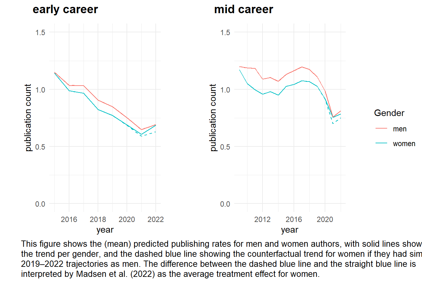

# now find a way to save correctly { pdf(file = './data/processed/20250729FigureRR2.pdf', width =
# 10, height =10) Figure_RR2 } dev.off() { png(file = './data/processed/20250729FigureRR2.png',
# width = 1600, height = 1600, units = 'px', res = 200) Figure_RR2 } dev.off()

Based on these figure we conclude that the ‘ATT’ for women is negative, women were less (negatively) impacted by COVID-19 than men.

---

Madsen, Emil Bargmann, Mathias Wullum Nielsen, Josefine Bjørnholm, Reshma Jagsi, and Jens Peter Andersen. 2022. “Author-Level Data Confirm the Widening Gender Gap in Publishing Rates During COVID-19.” eLife 11 (March). https://doi.org/10.7554/elife.76559.

---

Copyright © 2024- Jochem Tolsma